カプランマイヤー曲線からデータを復元する方法の学習記録(後編)

【学習動機】

前編からの続き.

moratoriamuo.hatenablog.com

カプランマイヤー曲線から, 疑似的な個々のtime-to-eventデータを復元したいとする. 復元の手順としては, Kaplan-Meier curve(カプランマイヤー曲線)からGraph Digitization Software(グラフ数値化ソフトウェア)を使ってグラフ上の各軸の値を取得して, その取得した値をGuyot et al. (2012) の提案したアルゴリズムを使って, 個々のtime-to-eventデータを復元していくことなる. 前編の記事では, digitize(digitise, 数値化)の方法について書いた.

今回の後編の記事では数値化したデータを使って, Guyot et al. (2012)の方法で復元していく方法について書く. コードはRを使う. Stataでやってみた文献( https://www.ncbi.nlm.nih.gov/pmc/articles/PMC5796634/ )もあるが, 今回は扱わない.

【学習内容】

Guyot et al. (2012)はこちら. Supplementary MaterialsにRのコードがある.

www.ncbi.nlm.nih.gov

Rのコードに合うように, 自分で前処理をしていく. このやり方が完全に正しい保証はないので, 使う場合は元文献にもあたって検証してから使用してください.

パッケージの読み込み.

library(tidyverse)
library(survival)
library(survminer)

前回の記事で作成したデータ(KM.csv)を読み込んで, 曲線の横棒の左端のみのデータになるように絞った後, それぞれの座標が, どの区間に該当するのかを変数(interval)にする. 最後に各座標に番号を付けておく.

df <- read_csv("KM.csv",
               col_names = c("Time", "Prob"),
               show_col_types = FALSE)

df2 <- df %>% 
  filter(row_number()%%2==1) %>% 
  mutate(
    interval = case_when(
      Time >= 0 & Time < 250 ~ 0,
      Time >= 250 & Time < 500 ~ 250,
      Time >= 500 & Time < 750 ~ 500,
      Time >= 750 & Time < 1000 ~ 750,
      Time >= 1000 ~ 1000
    ),
    rn = row_number()
  )

対象の文献でNumber at Riskの情報を読み込ませる.

df_NatRisk <- data.frame(
  interval = 1:5,
  Time = c(0, 250, 500, 750, 1000),
  NatRisk = c(228, 115, 41, 10, 2)
)

Guyot et al.(2012)のSupplementary Materialsのコードを改変しながら利用.

総イベント数が手に入る場合は記入する. 今回は総イベント数が分かっている(169)として扱う. 分からない場合はNAにする. 分かっている場合の方がもちろん復元の精度は良くなる. arm.idは今回は群分けしていないので, allとしている.

# 総イベント数が分からない場合はNA
tot.events <- "NA" #tot.events = total no. of events reported. If not reported, then tot.events="NA"
tot.events <- "169" # 総イベント数が分かる場合は記入
arm.id <- "all" #arm indicator

出来上がったデータセットをcsvファイルにするために, 名前を決めておく.

###FUNCTION INPUTS
KMdatafile <- "KMdata.csv" #Output file events and cens
KMdataIPDfile <- "KMdataIPD.csv" #Output file for IPD

元のコードに合わせるため, 変数を作成(もっと整理できそうだけれど今回は実行重視ということで).

t.S <- df2$Time
S <- df2$Prob
pub.risk <- df_NatRisk %>% 
  rename(
    t.risk = Time,
    n.risk = NatRisk
  ) 
t.risk <- pub.risk$t.risk
n.risk <- pub.risk$n.risk

Number at Riskの各区間に含まれるクリックの番号のlowerとupperの値を計算する. これはGuyot et al.(2012)のTable 2の不足分に該当. このあたりの計算は場当たり的に作成しているので, 状況に合わせて改変する必要があるかもしれない.

# 
lower <- numeric(nrow(pub.risk))
upper <- numeric(nrow(pub.risk))

for(i in 1:(length(t.risk)-1)){
  intvl <- 
    df2 %>% mutate(l = t.risk[i],
                   u = t.risk[i+1]) %>% 
    filter(l<=Time & Time<u)
  lower[i] <- min(intvl$rn)
  upper[i] <- max(intvl$rn)
  
  # 最後の区間だけ例外処理
  intvl <- 
    df2 %>% mutate(u=t.risk[i+1]) %>% 
    filter(u<=Time)
  lower[i+1] <- min(intvl$rn)
  upper[i+1] <- max(intvl$rn)
}

## Warning in min(intvl$rn): min の引数に有限な値がありません: Inf を返します

## Warning in max(intvl$rn): max の引数に有限な値がありません: -Inf を返します

Guyot et al.(2012)のTable 2を作成しなおす. ただし, この計算の仕方だと, たとえば, イベントが全く起きない区間があると, 上手く行かないことがあるので, そのときは臨機応変に対応する必要がある.

pub.risk <- 
  pub.risk %>% mutate(lower=lower, upper=upper) %>% 
  filter(!is.infinite(lower)) %>% 
  filter(!is.infinite(upper))
pub.risk

##   interval t.risk n.risk lower upper
## 1        1      0    228     1    56
## 2        2    250    115    57    92
## 3        3    500     41    93   114
## 4        4    750     10   115   118

アルゴリズムに必要な値の作成.

t.risk <- pub.risk$t.risk
n.risk <- pub.risk$n.risk
lower <- pub.risk$lower
upper <- pub.risk$upper

n.int <- length(n.risk)
n.t <- upper[n.int]

準備はできたので, Guyot et al.(2012)のアルゴリズムに従う.

#Initialise vectors
arm <- rep(arm.id,n.risk[1])
n.censor <- rep(0,(n.int-1))
n.hat <- rep(n.risk[1]+1,n.t)
cen <- rep(0,n.t)
d <- rep(0,n.t)
KM.hat <- rep(1,n.t)
last.i <- rep(1,n.int)
sumdL <- 0

if (n.int > 1){
  #Time intervals 1,...,(n.int-1)
  for (i in 1:(n.int-1)){
    #First approximation of no. censored on interval i
    n.censor[i] <- round(n.risk[i]*S[lower[i+1]]/S[lower[i]]- n.risk[i+1])
    #Adjust tot. no. censored until n.hat = n.risk at start of interval (i+1)
    while((n.hat[lower[i+1]]>n.risk[i+1])||((n.hat[lower[i+1]]<n.risk[i+1])&&(n.censor[i]>0))){
      if (n.censor[i]<=0){
        cen[lower[i]:upper[i]] <- 0
        n.censor[i] <- 0
      }
      if (n.censor[i]>0){
        cen.t<-rep(0,n.censor[i])
        for (j in 1:n.censor[i]){
          cen.t[j] <- t.S[lower[i]] +
            j*(t.S[lower[(i+1)]]-t.S[lower[i]])/(n.censor[i]+1)
        }
        #Distribute censored observations evenly over time. Find no. censored on each time interval.
        cen[lower[i]:upper[i]]<-hist(cen.t,breaks=t.S[lower[i]:lower[(i+1)]],
                                     plot=F)$counts
      }
      #Find no. events and no. at risk on each interval to agree with K-M estimates read from curves
      n.hat[lower[i]]<-n.risk[i]
      last <- last.i[i]
      for (k in lower[i]:upper[i]){
        if (i==1 & k==lower[i]){
          d[k] <- 0
          KM.hat[k] <- 1
        }
        else {
          d[k] <- round(n.hat[k]*(1-(S[k]/KM.hat[last])))
          KM.hat[k] <- KM.hat[last]*(1-(d[k]/n.hat[k]))
        }
        n.hat[k+1] <- n.hat[k]-d[k]-cen[k]
        if (d[k] != 0) last<-k
      }
      n.censor[i] <- n.censor[i]+(n.hat[lower[i+1]]-n.risk[i+1])
    }
    if (n.hat[lower[i+1]]<n.risk[i+1]) n.risk[i+1]<-n.hat[lower[i+1]]
    last.i[(i+1)] <- last
  }
}

#Time interval n.int.
if (n.int>1){
  #Assume same censor rate as average over previous time intervals.
  n.censor[n.int] <- min(round(sum(n.censor[1:(n.int-1)])*(t.S[upper[n.int]]-
                                                            t.S[lower[n.int]])/(t.S[upper[(n.int-1)]]-t.S[lower[1]])), n.risk[n.int])
}
if (n.int==1){n.censor[n.int]<-0}
if (n.censor[n.int] <= 0){
  cen[lower[n.int]:(upper[n.int]-1)]<-0
  n.censor[n.int] <- 0
}
if (n.censor[n.int]>0){
  cen.t<-rep(0,n.censor[n.int])
  for (j in 1:n.censor[n.int]){
    cen.t[j] <- t.S[lower[n.int]] +
      j*(t.S[upper[n.int]]-t.S[lower[n.int]])/(n.censor[n.int]+1)
  }
  cen[lower[n.int]:(upper[n.int]-1)] <- hist(cen.t,breaks=t.S[lower[n.int]:upper[n.int]],
                                           plot=F)$counts
}
#Find no. events and no. at risk on each interval to agree with K-M estimates read from curves
n.hat[lower[n.int]] <- n.risk[n.int]
last<-last.i[n.int]
for (k in lower[n.int]:upper[n.int]){
  if(KM.hat[last] !=0){
    d[k] <- round(n.hat[k]*(1-(S[k]/KM.hat[last])))} else {d[k]<-0}
  KM.hat[k] <- KM.hat[last]*(1-(d[k]/n.hat[k]))
  n.hat[k+1] <- n.hat[k]-d[k]-cen[k]
  #No. at risk cannot be negative
  if (n.hat[k+1] < 0) {
    n.hat[k+1] <- 0
    cen[k] <- n.hat[k] - d[k]
  }
  if (d[k] != 0) last<-k
}
#If total no. of events reported, adjust no. censored so that total no. of events agrees.
if (tot.events != "NA"){
  if (n.int>1){
    sumdL <- sum(d[1:upper[(n.int-1)]])
    #If total no. events already too big, then set events and censoring = 0 on all further time intervals
    if (sumdL >= tot.events){
      d[lower[n.int]:upper[n.int]] <- rep(0,(upper[n.int]-lower[n.int]+1))
      cen[lower[n.int]:(upper[n.int]-1)] <- rep(0,(upper[n.int]-lower[n.int]))
      n.hat[(lower[n.int]+1):(upper[n.int]+1)] <- rep(n.risk[n.int],(upper[n.int]+1-lower[n.int]))
    }
  }
  #Otherwise adjust no. censored to give correct total no. events
  if ((sumdL < tot.events)|| (n.int==1)){
    sumd<-sum(d[1:upper[n.int]])
    while ((sumd > tot.events)||((sumd< tot.events)&&(n.censor[n.int]>0))){
      n.censor[n.int] <- n.censor[n.int] + (sumd - tot.events)
      if (n.censor[n.int]<=0){
        cen[lower[n.int]:(upper[n.int]-1)]<-0
        n.censor[n.int] <- 0
      }
      if (n.censor[n.int]>0){
        cen.t <- rep(0,n.censor[n.int])
        for (j in 1:n.censor[n.int]){
          cen.t[j] <- t.S[lower[n.int]] +
            j*(t.S[upper[n.int]]-t.S[lower[n.int]])/(n.censor[n.int]+1)
        }
        cen[lower[n.int]:(upper[n.int]-1)]<-hist(cen.t,breaks=t.S[lower[n.int]:upper[n.int]],
                                                 plot=F)$counts
      }
      n.hat[lower[n.int]]<-n.risk[n.int]
      last <- last.i[n.int]
      for (k in lower[n.int]:upper[n.int]){
        d[k] <- round(n.hat[k]*(1-(S[k]/KM.hat[last])))
        KM.hat[k] <- KM.hat[last]*(1-(d[k]/n.hat[k]))
        if (k != upper[n.int]){
          n.hat[k+1] <- n.hat[k]-d[k]-cen[k]
          #No. at risk cannot be negative
          if (n.hat[k+1] < 0) {
            n.hat[k+1] <- 0
            cen[k] <- n.hat[k] - d[k]
          }
        }
        if (d[k] != 0) last<-k
      }
      sumd <- sum(d[1:upper[n.int]])
    }
  }
}

write.csv(matrix(c(t.S,n.hat[1:n.t],d,cen),ncol=4,byrow=F),
          paste("output/",KMdatafile,sep=""))

### Now form IPD ###
#Initialise vectors
t.IPD <- rep(t.S[n.t],n.risk[1])
event.IPD <- rep(0,n.risk[1])
#Write event time and event indicator (=1) for each event, as separate row in t.IPD and event.IPD
k=1
for (j in 1:n.t){
  if(d[j]!=0){
    t.IPD[k:(k+d[j]-1)] <- rep(t.S[j],d[j])
    event.IPD[k:(k+d[j]-1)] <- rep(1,d[j])
    k <- k+d[j]
  }
}
#Write censor time and event indicator (=0) for each censor, as separate row in t.IPD and event.IPD
for (j in 1:(n.t-1)){
  if(cen[j]!=0){
    t.IPD[k:(k+cen[j]-1)] <- rep(((t.S[j]+t.S[j+1])/2),cen[j])
    event.IPD[k:(k+cen[j]-1)] <- rep(0,cen[j])
    k <- k+cen[j]
  }
}

復元によって得られた, 疑似的なtime-to-eventデータの個票データを作成する.

#Output IPD
IPD <- matrix(c(t.IPD,event.IPD,arm),ncol=3,byrow=F)
#Find Kaplan-Meier estimates
IPD <- IPD %>% as.data.frame() %>% 
  set_names(c("time","event","arm")) %>% 
  mutate(time=as.numeric(time),
         event=as.numeric(event))

write.csv(IPD, str_c("output/",KMdataIPDfile), row.names = FALSE)

疑似的な個票データはこのような感じ.

head(IPD)

##        time event arm
## 1  5.847953     1 all
## 2  5.847953     1 all
## 3  5.847953     1 all
## 4 11.695906     1 all
## 5 13.157895     1 all
## 6 14.619883     1 all

復元によって得られたデータでカプランマイヤー推定をする. 総イベント数を指定しているので一致する. 指定できないと一致するとは限らない.

KM.est <- survfit(Surv(time,event)~1,
                data = IPD,
                type = "kaplan-meier",)
KM.est

## Call: survfit(formula = Surv(time, event) ~ 1, data = IPD, type = "kaplan-meier")
## 
##        n events median 0.95LCL 0.95UCL
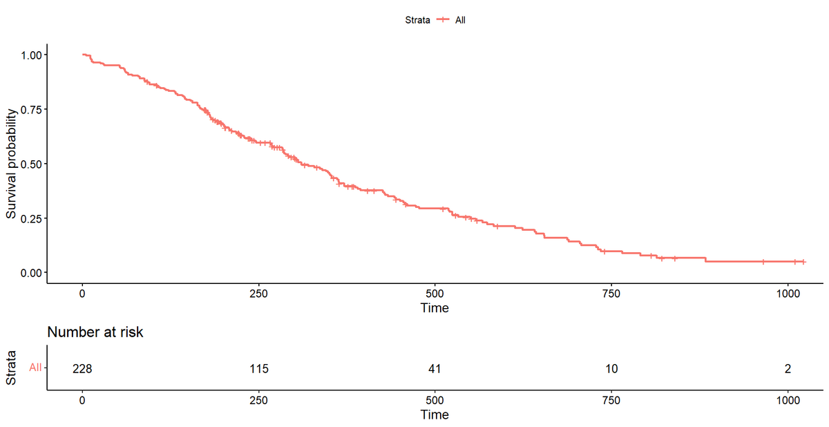
## [1,] 228    169    310     285     364

曲線を描いてみる.

ggsurvplot(KM.est, 
           data = IPD,
           conf.int = FALSE,
           risk.table = TRUE)

元データのカプランマイヤー曲線は

であり, もちろん完全再現ではないが, 近いものが復元できている(と思う).

最後に繰り返しになるが, このやり方が完全に正しい保証はないので, 使う場合は元文献にもあたって検証してから使用してください.

【学習予定】

Rには{reconstructKM}というパッケージがあるが, こちらはあまり読み込んでいない. https://cran.r-project.org/web/packages/reconstructKM/index.html

他にもっといいやり方があるかもしれないので, 見つけたら学習する.

霞と側杖を食らう

ほしいものです。なにかいただけるとしあわせです。[https://www.amazon.jp/hz/wishlist/ls/2EIEFTV4IKSIJ?ref_=wl_share]

カプランマイヤー曲線からデータを復元する方法の学習記録(後編)

【学習動機】

【学習内容】

【学習予定】